Easy Way to Delete Duplicates in Excel
Removing both duplicates in Excel is a common thing while we merge or combine multiple worksheets data. As a result, identical entries exist throughout multiple worksheets. These identical or duplicates pose calculation issues in Excel. In this article, we demonstrate multiple ways to remove both duplicates in Excel.
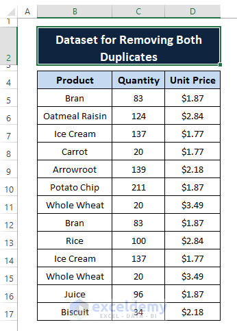
Let's say after merging two worksheets' data we have a dataset that contains identical entries. We can remove those identical entries or both duplicates using a Helper Column, Formula (i.e., combining IF and COUNTIF functions), Conditional Formatting, and VBA Macro Code.
Download Excel Workbook
5 Easy Ways to Remove Both Duplicates in Excel
Method 1: Using a Helper Column to Remove Both Duplicates in Excel
From the dataset, we notice the occurrences of duplicates among entries (depicted in the below screenshot). And we want both duplicates to be removed.
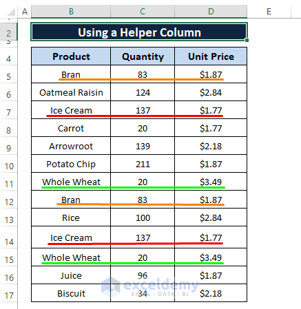
To do so, we can use a helper column to identify both duplicates and sort them to display entries that have no duplicates.
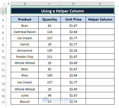
Step 1: Insert a Helper Column (i.e., Column E) adjacent to the raw dataset's columns.
Step 2: Paste the following formula in any cell (i.e., E5).
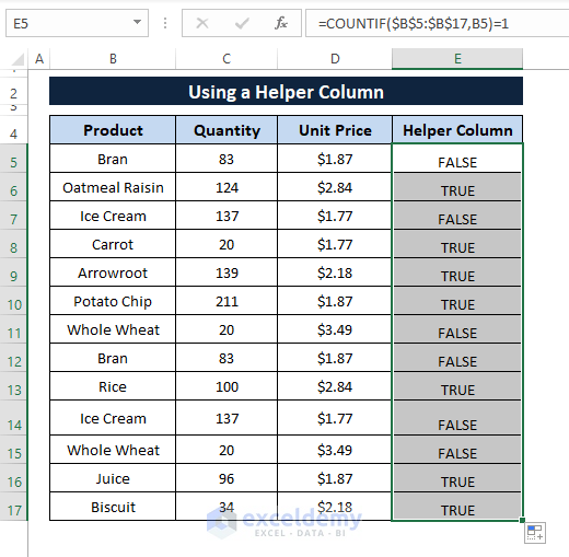
=COUNTIF($B$5:$B$17,B5)=1
The formula counts cells in the B5:B17 range that match the criteria B5 and returns TRUE (if the cell satisfies the criteria) or FALSE (if the cell does not satisfy the criteria).
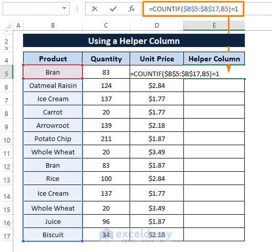
Step 3: Press ENTER and Drag the Fill Handle to display TRUE or FALSE in all the cells as depicted in the following image.
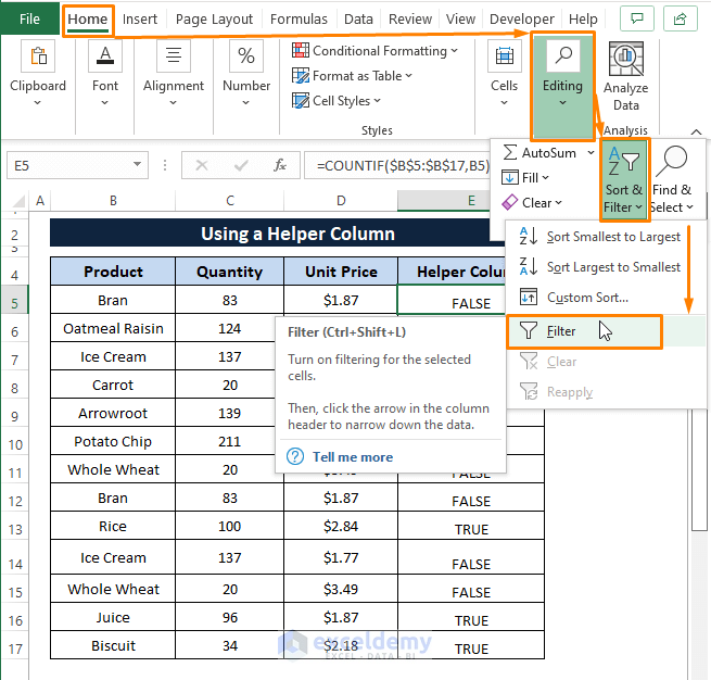
Step 4: Now, Go to the Home Tab > Select Sort & Filter (from the Editing section) > Choose Filter (from the options).
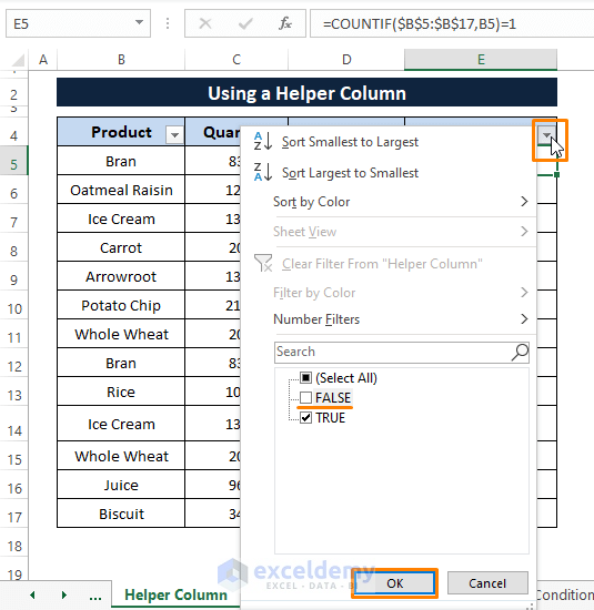
Step 5: The Filter icon appears on all the column headers.
Click on the Filter Icon on the Helper Column header (the apply Filter window appears).
Unselect the FALSE option in the apply Filter window.
Click OK.
The consequences of unselecting the FALSE option result in a scenario similar to the picture below.
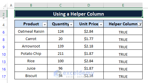
You can modify the formula applied in the Helper Column to display your desired outcome.
Method 2: Using a Formula to Remove Both Duplicates in Excel
Similar to Method 1, we can insert a customized formula in any adjacent column to indicate duplicates. In this case, we use IF and COUNTIF functions to develop a customized formula and display any character to showcase the duplicates.
Step 1: Add a helper column and Type the below formula in any blank cell (i.e., E5).
=IF(COUNTIF($B$5:$B$17,B5)=1,1,0)
The formula performs a logical test (i.e., COUNTIF($B$5:$B$17,B5)=1) where the COUNTIF function returns TRUE or FALSE applying the criteria (i.e., B5) in the range (i.e., B5:B17). Then the IF function returns 1 or 0 if a cell satisfies the criteria or not respectively.
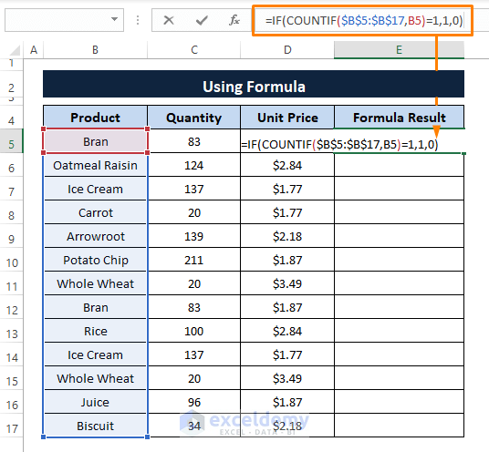
Step 2: Hit ENTER afterward Drag the Fill Handle to display 1 or 0's in the cells.
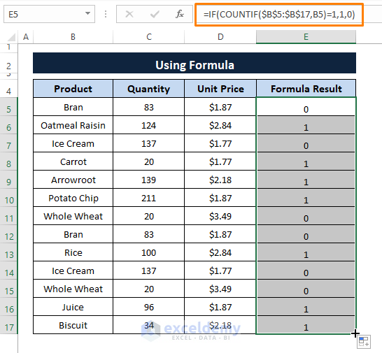
Step 3: Apply the Filter feature as done in Step 4 of Method 1.
Then Click on the Filter icon of the Formula Result column header.
Unselect option 0.
And Click OK.
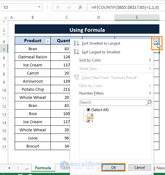
In a moment all the 0's get removed and only the entries that have no duplicates remain as shown in the below picture.
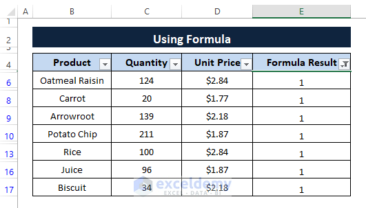
According to the formula (i.e., =IF(COUNTIF($B$5:$B$17,B5)=1,1,0 )) 1 indicates entries that have no identical entries and 0 indicates entries that have identical entries.
Method 3: Using Conditional Formatting (Highlight Duplicates)
In Excel, Conditional Formatting is one of the common ways to highlight duplicates. In this method, we demonstrate how we can use Conditional Formatting to color format cells in a dataset after that sort and remove them using any convenient options.
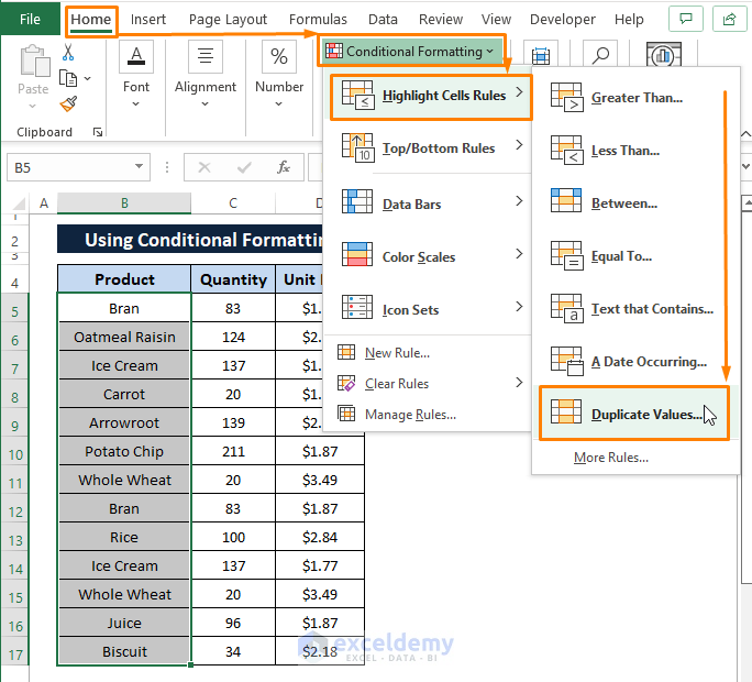
Step 1: Select the range (i.e., B5:B17) you want to apply Conditional Formatting.
Hover to the Home tab > Select Conditional Formatting > Select Highlight Cells Rules > Choose Duplicate Values.
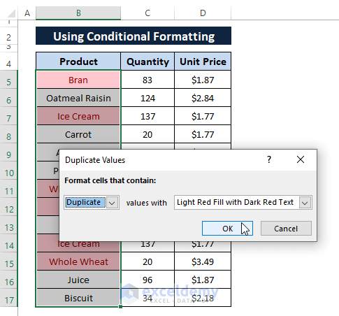
Step 2: The Duplicate Values window appears. In the Duplicate Values window,
Choose Duplicate (under the Formats cells that contain note's 1st box).
Select any Cell Color (i.e., Light Red Fill with Dark Red Text) in the 2nd box.
Click OK.
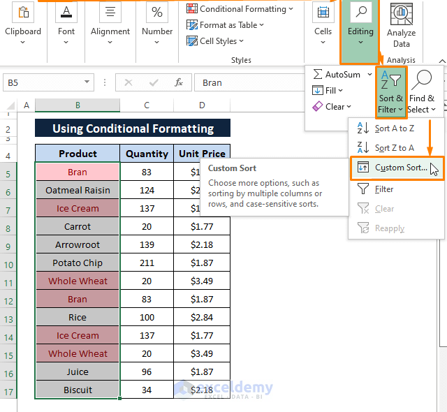
Step 3: Go to the Home tab > Select Sort & Filter (from the Editing section) > Choose Custom Sort (the Sort window appears).
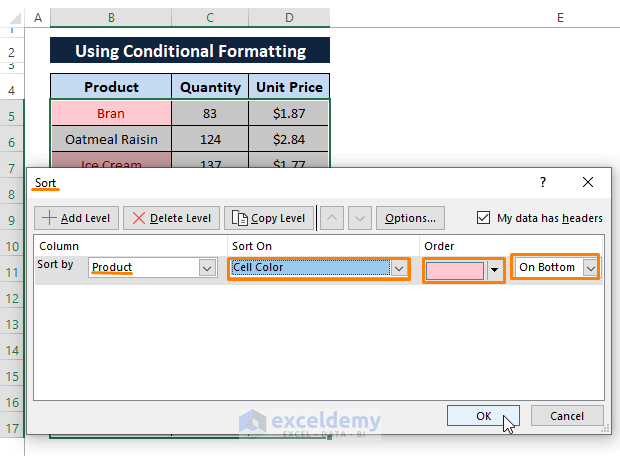
Step 4: In the Sort window,
Select Product (under Column) as Sort by option.
Select Cell Color (under Sort On).
Select the Color under Order.
Choose On Bottom to display the duplicates at the bottom.
Click OK.
All the duplicates sit at the bottom of the dataset as depicted in the below screenshot.
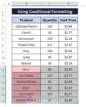
However, to remove the color formatted duplicates we can follow three ways. They are a) Delete feature, b) Keyboard Shortcuts (CTRL+-), and c) Context Menu Delete option.
a) Delete feature
➤ Select the color formatted cells' range. Then, Go to the Home tab > Select Delete (from Cells section) > Select Delete Sheet Rows.
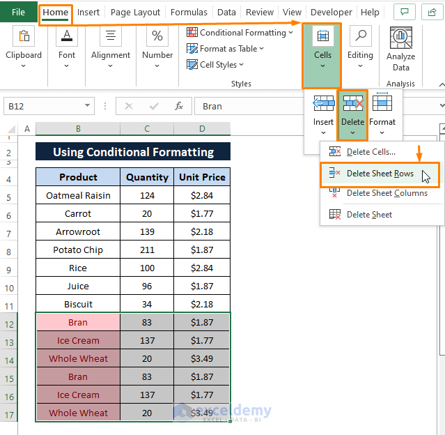
The Delete Sheet Rows option deletes all the selected rows as depicted in the following image.
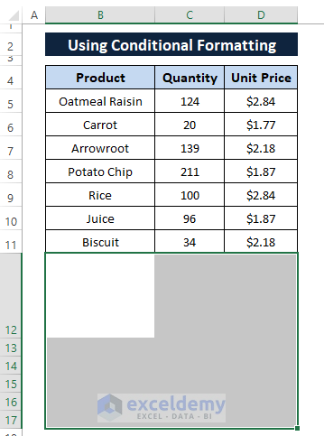
b) Keyboard Shortcuts (CTRL+-)
➤ After selecting the color formatted rows, press CTRL+- altogether. It brings out the Delete window as you see in the latter screenshot.
Select the Entire Row option.
Click OK.
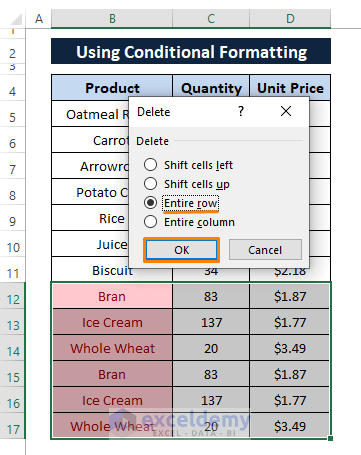
Clicking OK deletes all the color-formatted cells as shown in the image below.

➤ Select the formatted cells' range then, right-click on them. The Context Menu appears.
In the Context Menu, Select Delete.
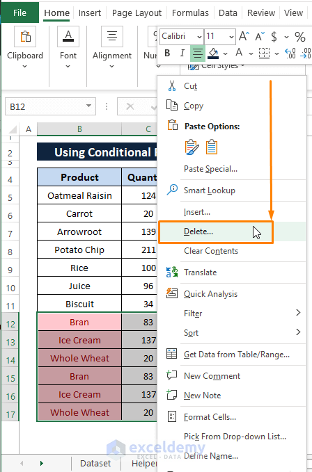
➤ The Delete window pops up. In the Delete window,
Select the Entire row option.
Click OK.

By Clicking OK you get all the color formatted cells removed similar to the picture below.

Method 4: Using Conditional Formatting (New Rule to Apply Color Format)
Identical to Method 3, in this method, we apply the color formatting to cell entries using Conditional Formatting. However, we apply a formula to color format the cells in the Conditional Formatting option. The Conditional Formatting colors format the cells if the formula returns TRUE for the cells.
Step 1: Go to the Home tab > Select Conditional Formatting > Choose New Rule (from the options).
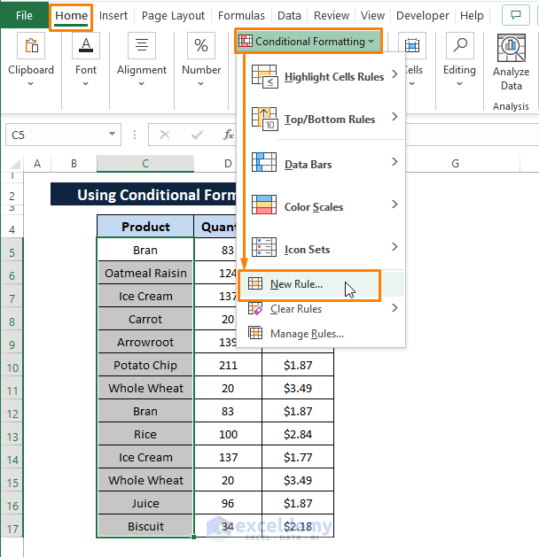
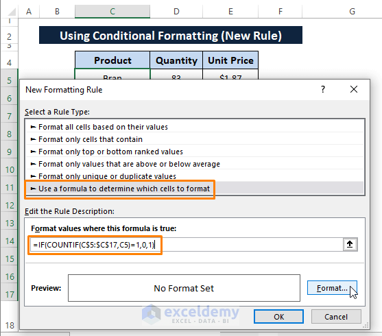
Step 2: The New Formatting Rule window appears. In the New Formatting Rule window,
Select Use a formula to determine which cells to format as Select a Rule Type.
Paste the following formula under Format values where this formula is true.
=IF(COUNTIF($C$5:$C$17,C5)=1,0,1)
This formula declares the same arguments as it does in Step 2 of Method 1 except returns 0 or 1 if entries satisfy the argument or not respectively.
Click on Format (the Format Cells window appears).
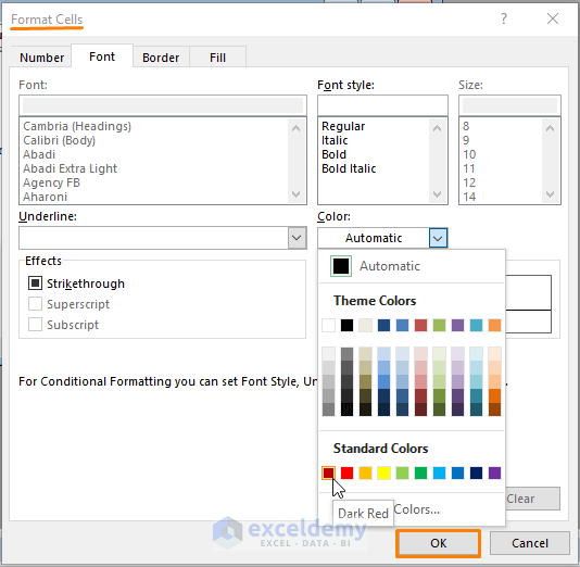
Step 3: In the Format Cells window, Select the Font color (i.e., Dark Red).
Click OK.
Step 4: By clicking OK in Step 3, you get back to the New Formatting Rule window again.
Click OK.

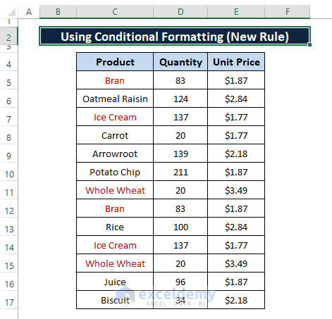
Step 4 applies the formula to the selection and colors format of the cells as you can see in the below depiction.
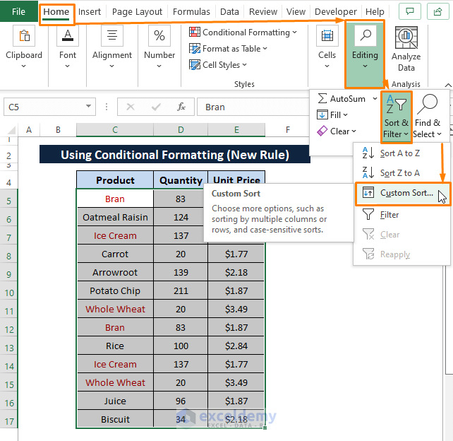
Step 5: To apply Sorting, Select the entire dataset then Go to the Home tab > Select Sort & Filter(from the Editing section) > Choose Custom Sort (from the options). The Sort window appears.
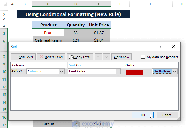
Step 6: Inside the Sort window,
Pick Column C (under Column) as Sort by option.
Choose Font Color (under Sort On).
Take the Color under Order.
Choose On Bottom to make the duplicates appear at the bottom.
Afterward, Click OK.
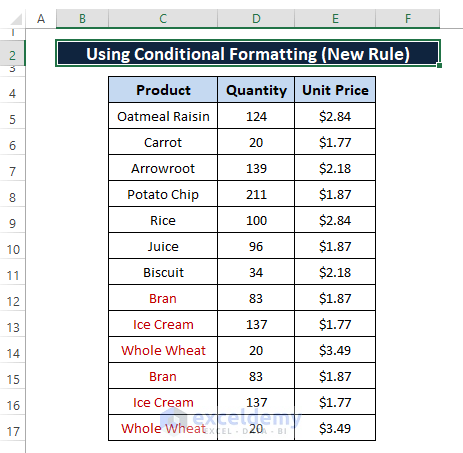
Font color formatted cells are placed at the bottom as shown in the below picture.
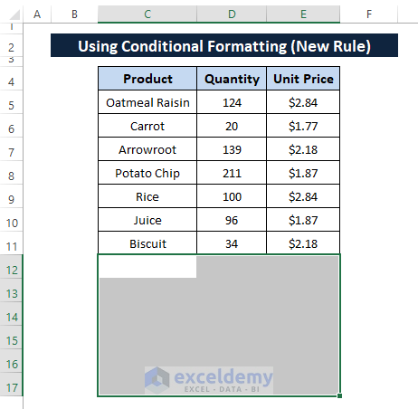
Step 7: Follow any Delete ways described in Method 3 and you'll get the same result as depicted below.
Method 5: Using VBA Macro Code
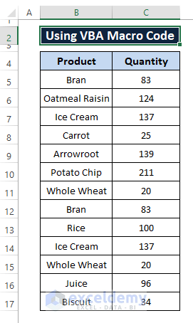
Excel VBA Macro Code also removes both duplicates if we instruct it to do so. Let's say, we consider only two columns (i.e., Product and Quantity) from where we remove all the duplicates.
So, we have a dataset something like the below image.
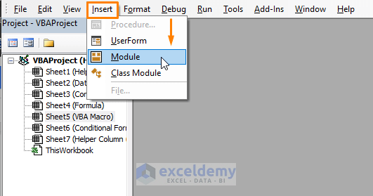
Step 1: Press ALT+F11 to open the Microsoft Visual Basic window. In the Microsoft Visual Basic Window, Select Insert > Choose Module to insert a Module in the Microsoft Visual Basic window.
Step 2: Paste the following code in the Module to remove all the duplicates from the dataset.
Sub Remove_Both_Duplicates() Dim Cell As Range With ActiveSheet.UsedRange For Each Cell In .Cells If Cell.Value <> "" And Application.CountIf(.Cells, Cell.Value) > 1 Then .Replace Cell.Value, "", xlWhole, , , , False, False End If Next On Error GoTo NoBlanks End With NoBlanks: End Sub 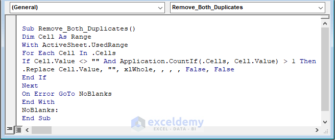
In the macro code, the COUNTIF function counts cells that have occurrences of more than 1. And the REPLACE function replaces the cells with blank strings.
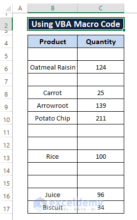
Step 3: Hit F5 to run the macro. Return to the worksheet and you see both duplicates get removed as displayed in the below picture.
Conclusion
In this article, we use Customized Formula, Conditional Formatting, and VBA Macro Code to remove both duplicates in Excel. As all the methods remove both duplicates; it's quite risky to apply these methods in a dataset if you want to maintain the ingenuity of the dataset. Otherwise, all described methods are super handy in removing both duplicates. I hope this article helps you to tidy your dataset by removing both duplicates. Comment if you have further inquiries or have anything to add.
Source: https://www.exceldemy.com/remove-both-duplicates-in-excel/
0 Response to "Easy Way to Delete Duplicates in Excel"
Post a Comment